Downloading and plotting Spanish temperatures with R

The idea of this post is to give an idea of three important tasks in any analysis of climate variables. i) obtaining the data from a reliable source, ii) cleaning those data and selecting the variables that may be of interest and iii) visualising those data. Here I try to present a clean and replicable code. Of course, like any script, it can be improved. I hope you like it.

Load R packages

library(reshape2)
library(tidyverse)
library(PupillometryR)
library(climaemet)
library(ggpubr)

Get api key from AEMET (Spanish metereological service)

browseURL("https://opendata.aemet.es/centrodedescargas/obtencionAPIKey")
aemet_api_key("YOUR API", 
              install = TRUE)

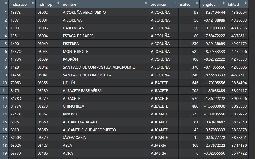
See all (of this package) AEMET stations

stations <- aemet_stations() 

Download monthly mean of the maximun temperatures using climaemet (See https://ropenspain.github.io/climaemet/index.html)

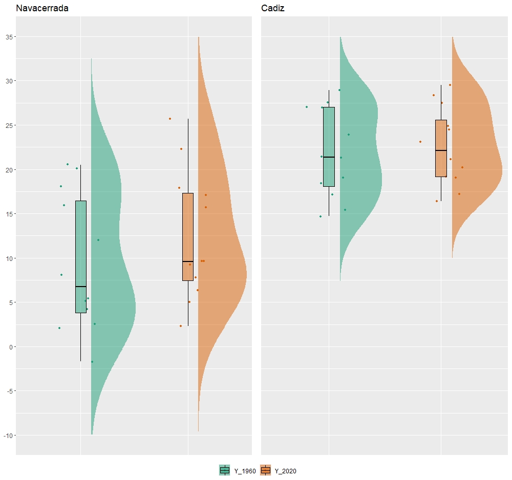
Here we will work with two very different weather stations, one in Cadiz (0 masl) and one in Navacerrada (1894 masl) to try to understand if temperature changes are homogeneous in different places.

station <- "2462" 

navacerrada_data <- tibble(monht = c(seq(1, 12, 1)))           # Create an empty data frame to store the data we are interested in.
for (y in c(1960, 2020)){                                      # Loop to select different years to see temperature differences
  data <- aemet_monthly_clim(station, year = y)                # Use the climemet function to download the data.
  data <- select(data, tm_max)                                 # Select the variable of interest. Monthly average of maximum temperatures
  names(data) <- paste0("Y_",y)                                # Rename variables to call them Y_1960 and Y_2020
  navacerrada_data <- cbind(navacerrada_data, data[c(1:12),])  # Join the downloaded data with the previously generated dataframe by columns.
}

navacerrada_data <- melt(navacerrada_data[,c(2,3)])            # Change the structure of the data in order to be able to graph it.

station <- "5973" 

cadiz_monthly <- tibble(monht = c(seq(1, 12, 1)))
for (y in c(1960, 2020)){
  data <- aemet_monthly_clim(station, year = y)
  data <- select(data, tm_max)
  names(data) <- paste0("Y_",y)
  cadiz_monthly <- cbind(cadiz_monthly, data[c(1:12),])
}


cadiz_data <- melt(cadiz_monthly[,c(2,3)])

After generating and cleaning the data, it is time for the long awaited moment. Let’s plot them with a bit of “statistical” art.

navacerrada <- ggplot(navacerrada_data,
                      aes(
                        x = variable,
                        y = value,
                        fill = variable,
                        colour = variable
                      )) +
  geom_flat_violin(
    position = position_nudge(x = .1, y = 0),
    trim = FALSE,
    alpha = 0.5,
    colour = NA
  ) +
  geom_point(position = position_jitter(width = .2),
             size = 2,
             shape = 20) +
  geom_boxplot(
    outlier.shape = NA,
    alpha = .5,
    width = .1,
    colour = "black"
  ) +
  scale_y_continuous("ºC",c(-10,-5,0,5,10,15,20,25,30,35), limits = c(-10,35))+
  scale_colour_brewer(palette = "Dark2") +
  scale_fill_brewer(palette = "Dark2") +
  ggtitle("Navacerrada") +
  theme(
    legend.title = element_blank(),
    axis.title.x = element_blank(),
    axis.text.x = element_blank(),
    axis.title.y = element_blank(),
    axis.ticks.x = element_blank()
  )


cadiz <-
  ggplot(cadiz_data,
         aes(
           x = variable,
           y = value,
           fill = variable,
           colour = variable
         )) +
  geom_flat_violin(
    position = position_nudge(x = .1, y = 0),
    trim = FALSE,
    alpha = 0.5,
    colour = NA
  ) +
  geom_point(position = position_jitter(width = .2),
             size = 2,
             shape = 20) +
  geom_boxplot(
    outlier.shape = NA,
    alpha = .5,
    width = .1,
    colour = "black"
  ) +
  scale_y_continuous("ºC",c(-10,-5,0,5,10,15,20,25,30,35), limits = c(-10,35))+
  scale_colour_brewer(palette = "Dark2") +
  scale_fill_brewer(palette = "Dark2") +
  ggtitle("Cadiz") +
  theme(
    legend.title = element_blank(),
    axis.title.x = element_blank(),
    axis.text.x = element_blank(),
    axis.ticks.x = element_blank(),
    axis.title.y = element_blank(),
    axis.text.y = element_blank(),
    axis.ticks.y = element_blank()
  )

ggarrange(navacerrada, cadiz, common.legend = TRUE, legend = "bottom")

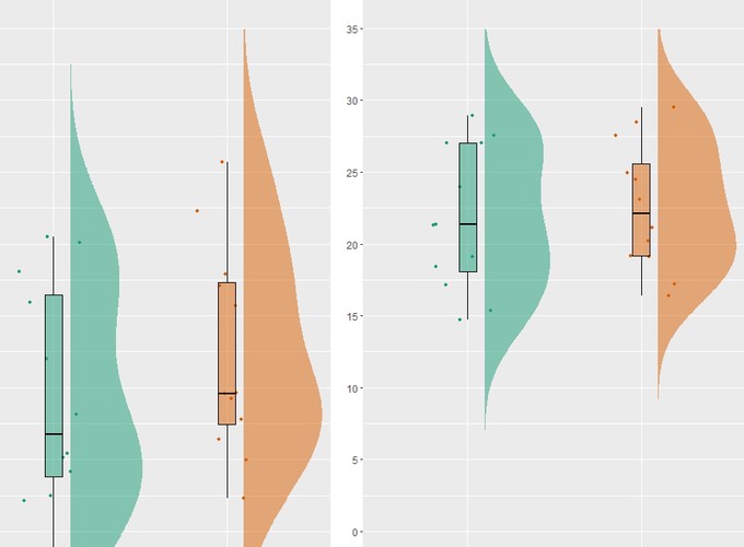
Here you can see the final result. As you can see the temperature changes have not followed the same pattern … Think about it …